Temperature of European rivers and future climate in 50 lines of R code

During the last summer the water temperature in some important rivers (especially the Rhine and the Rhone) in central Europe was so high that some nuclear and coal power plants in Germany, France and Switzerland had to limit their generation or even shut down due to the regulations imposing them to do not discharge the warm water used for cooling the plant when the river temperature was too high. It was July, during a heatwave strong enough to deserve a Wikipedia page.

Now the question: what is going to happen in the next decades? How much the global warming affect the temperature of those rivers? To answer this question you need three things:

1. Water data: month average of river temperature data for all the emissions scenario and all the future periods available on the Copernicus Climate Data Store (if you don’t have an account you can register here, it’s free) and you also need the definition of the sub-basins used by the model, unfortunately not bundled with the Copernicus data, available on Zenodo.

2. River data: a shapefile with the major European river is available on the rich website of the European Environment Agency. This one should be ok but in principle you can use any shapefile you have available.

3. A R working environment with the tidyverse, the simple features (sf) package and the ncdf4 package

Good for us all the data and the software is open: the CDS data is licensed for reproduction; distribution; communication to the public; adaptation, modification and combination with other data, the data on Zenodo is under CC BY 4.0 license and the data on the EEA website has a re-use policy. R and all the packages are instead under GPL license.

Ok, we are ready to go.

Let’s start loading the package we needs into our R environment.

library(sf)
## Linking to GEOS 3.6.1, GDAL 2.1.3, proj.4 4.9.3
library(tidyverse)
## ── Attaching packages ────────────────────────────── tidyverse 1.2.1 ──
## ✔ ggplot2 3.0.0     ✔ purrr   0.2.5
## ✔ tibble  1.4.2     ✔ dplyr   0.7.7
## ✔ tidyr   0.8.1     ✔ stringr 1.3.1
## ✔ readr   1.1.1     ✔ forcats 0.3.0
## ── Conflicts ───────────────────────────────── tidyverse_conflicts() ──
## ✖ dplyr::filter() masks stats::filter()
## ✖ dplyr::lag()    masks stats::lag()
library(ncdf4)

Before choosing the river we want to analyse, we need to load both the river Shapefile and the definition of the sub-basins. I assume that you have extracted all the data into the data folder.

subbasins_definition <- st_read('data/EHYPE3_subbasins.shp')
## Reading layer `EHYPE3_subbasins' from data source `/Users/matteodefelice/Documents/Work/swicca-rivers/data/EHYPE3_subbasins.shp' using driver `ESRI Shapefile'
## Simple feature collection with 35408 features and 2 fields
## geometry type:  MULTIPOLYGON
## dimension:      XY
## bbox:           xmin: -24.56223 ymin: 29.00417 xmax: 66.59261 ymax: 71.18595
## epsg (SRID):    4326
## proj4string:    +proj=longlat +datum=WGS84 +no_defs
rivers <- st_read('data/Large_rivers.shp')
## Reading layer `Large_rivers' from data source `/Users/matteodefelice/Documents/Work/swicca-rivers/data/Large_rivers.shp' using driver `ESRI Shapefile'
## Simple feature collection with 20 features and 2 fields
## geometry type:  MULTILINESTRING
## dimension:      XY
## bbox:           xmin: 2683612 ymin: 1681231 xmax: 5852419 ymax: 5050981
## epsg (SRID):    NA
## proj4string:    +proj=laea +lat_0=52 +lon_0=10 +x_0=4321000 +y_0=3210000 +ellps=GRS80 +units=m +no_defs

Into the rivers data frame you have the spatial data for the 20 longest rivers in Europe.

head(rivers)
## Simple feature collection with 6 features and 2 fields
## geometry type:  MULTILINESTRING
## dimension:      XY
## bbox:           xmin: 2764964 ymin: 1681231 xmax: 5852419 ymax: 3422320
## epsg (SRID):    NA
## proj4string:    +proj=laea +lat_0=52 +lon_0=10 +x_0=4321000 +y_0=3210000 +ellps=GRS80 +units=m +no_defs
##           NAME Shape_Leng                       geometry
## 1       Danube  2770357.4 MULTILINESTRING ((4185683 2...
## 2        Douro   816245.2 MULTILINESTRING ((2764964 2...
## 3         Ebro   826990.9 MULTILINESTRING ((3178372 2...
## 4         Elbe  1087288.3 MULTILINESTRING ((4235352 3...
## 5 Guadalquivir   599758.3 MULTILINESTRING ((2859329 1...
## 6     Guadiana  1063055.4 MULTILINESTRING ((2778234 1...

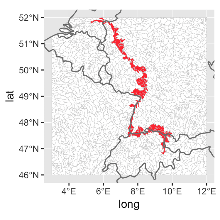
We are ready to choose the river we want to analyse, let’s focus on the Rhine.

selected_river <- rivers %>%
    filter(str_detect(NAME, 'Rhine'))

What we need now? We need to extract the vector of all the sub-basins identifiers - stored in the field SUBID of the subbasins_definition shapefile - of the sub-basins that include the selected river. To do that we should intersect the two shapefiles after having them in the same coordinate reference system (crs)

sel_subids <- st_intersection(selected_river %>% st_transform(st_crs(subbasins_definition)),
                              subbasins_definition) %>%
    pull(SUBID)
## although coordinates are longitude/latitude, st_intersection assumes that they are planar
## Warning: attribute variables are assumed to be spatially constant
## throughout all geometries

We can show the selected sub-basins to check if everything is correct. The plot takes a few seconds, because the shapefile of the sub-basins is quite large.

check_plot <- subbasins_definition %>% 
    transmute(selected = if_else(SUBID %in% sel_subids, 1, 0)) %>% 
    st_crop(c(xmin = 3, ymin = 46, xmax = 12, ymax = 52)) %>% 
    ggplot() + 
    geom_sf(aes(fill = as.factor(selected)), lwd = 0.1, color = 'gray80') +  
    borders("world") + 
    coord_sf(xlim = c(3, 12), ylim = c(46, 52)) + 
    scale_fill_manual(values = c('white','brown1'), guide = FALSE) 
## although coordinates are longitude/latitude, st_intersection assumes that they are planar
## Warning: attribute variables are assumed to be spatially constant
## throughout all geometries
## 
## Attaching package: 'maps'
## The following object is masked from 'package:purrr':
##
print(check_plot)

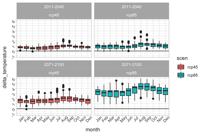
Now it’s time to load the climate data. For the sake of conciseness, I will limit the analysis to the scenarios R85 and R45 and only to the first 4 models, unfortunately the NetCDFs need a bit of data wrangling to be used in an efficient way.

target_scenario <- c('rcp45', 'rcp85')
target_periods  <- c('2011-2040', '2071-2100')
model_data <- tibble() 
for (scenario in target_scenario) {
    for (period in target_periods) {
    netcdf_file <- nc_open(paste0('data/wtemp-periodmonavg_abs_EUR-44_', scenario, '_IMPACT2C_QM-EOBS_', period, '_1971-2000_remap215.nc'))
    subid <- ncvar_get(netcdf_file, 'id')
    mask <- subid %in% sel_subids
    model_data = bind_rows(
        model_data,
        ncvar_get(netcdf_file, 'variable1')[mask,] %>% as_tibble() %>% set_names(month.abb) %>% mutate(model = 'm1', scen = scenario, per = period),
        ncvar_get(netcdf_file, 'variable2')[mask,] %>% as_tibble() %>% set_names(month.abb) %>% mutate(model = 'm2', scen = scenario, per = period),
        ncvar_get(netcdf_file, 'variable3')[mask,] %>% as_tibble() %>% set_names(month.abb) %>% mutate(model = 'm3', scen = scenario, per = period),
        ncvar_get(netcdf_file, 'variable4')[mask,] %>% as_tibble() %>% set_names(month.abb) %>% mutate(model = 'm4', scen = scenario, per = period)
    ) 
    nc_close(netcdf_file)
    }
}

Now model_data contains all the change of temperatures of all the 12 months for all the sub-basins for the Rhine river according to four different climate models for two scenarios (in the CDS dataset page you can find a detailed documentation explaining everything). Before the final plot, we must make model_data tidier and give to the factors describing the months the proper order instead of the alphabetic one.

tidy_model_data <- model_data %>%
    gather(month, delta_temperature, -model, -per, -scen) %>% 
    mutate(month = fct_relevel(month, month.abb))
head(tidy_model_data)
## # A tibble: 6 x 5
##   model scen  per       month delta_temperature
##   <chr> <chr> <chr>     <fct>             <dbl>
## 1 m1    rcp45 2011-2040 Jan               0.400
## 2 m1    rcp45 2011-2040 Jan               0.400
## 3 m1    rcp45 2011-2040 Jan               0.600
## 4 m1    rcp45 2011-2040 Jan               0.600
## 5 m1    rcp45 2011-2040 Jan               0.600
## 6 m1    rcp45 2011-2040 Jan               0.700

Now we can plot - using ggplot2 - the expected change in monthly temperature for the two periods and the two scenarios. We are using a boxplot because we are considering all the 109 sub-basins that contain the Rhine river.

ggplot(tidy_model_data , aes(x = month, y = delta_temperature, fill = scen)) + 
    geom_boxplot(aes(group = month), position=position_dodge(width=.60)) + 
    geom_hline(yintercept = 0) +
    facet_wrap(per~scen) +
    scale_y_continuous(breaks = seq(-1, 9, 1), limits = c(-1, 6)) +
    theme_light() +
    theme(axis.text = element_text(angle = 45))
## Warning: Removed 65 rows containing non-finite values (stat_boxplot).