Consecutive days of good weather in the Netherlands
I have recently moved in North Holland and in the past weeks the weather was particularly fortunate: for many (consecutive) days there was no rain and the temperature have been very high for this area (the maximum temperature was easily above 25° degrees).
Given that I have no experience yet for this weather, I asked around how frequently this happens and I got diverse answers. Then, I have decided to look at some historical time-series of temperature and precipitation to try to satisfy my curiosity.
Firstly, I have downloaded the data of the weather stations part of the ECA (European Climate Assessment) dataset. The dataset is freely available for non-commercial research and education. In the North Holland area there are 4-5 suitable weather stations and I opted for the one from Schiphol, which is the longest one with the data starting in 1951 (temperature, precipitation data is even longer). To give you an idea, this is the list of the stations providing maximum temperature data available in the latest release of the dataset (17.0).
To carry out the analysis I have used the core
Tidyverse R packages and lubridate (one
non-core tidyverse package) plus zoo.
library(lubridate)
library(tidyverse)
library(zoo)
I have downloaded two large zip files containing all the station data
for precipitation (rr) and maximum temperature (tx) and from them I
have selected the files for Schiphol. I have loaded them into memory with the following lines:
read_station <- function(filename) {
    read_csv(filename,
    col_types = cols(DATE = col_datetime(format = "%Y%m%d")),
    skip = 20
    )
}
station_files <- c("RR_STAID000593.txt", "TX_STAID000593.txt") # SCHIPHOL (NL)
print(read_station(station_files[1]))

## # A tibble: 55,273 x 5
##    STAID SOUID DATE                   RR  Q_RR
##    <int> <int> <dttm>              <int> <int>
##  1   593   503 1866-12-01 00:00:00 -9999     9
##  2   593   503 1866-12-02 00:00:00 -9999     9
##  3   593   503 1866-12-03 00:00:00 -9999     9
##  4   593   503 1866-12-04 00:00:00 -9999     9
##  5   593   503 1866-12-05 00:00:00 -9999     9
##  6   593   503 1866-12-06 00:00:00 -9999     9
##  7   593   503 1866-12-07 00:00:00 -9999     9
##  8   593   503 1866-12-08 00:00:00 -9999     9
##  9   593   503 1866-12-09 00:00:00 -9999     9
## 10   593   503 1866-12-10 00:00:00 -9999     9
## # ... with 55,263 more rows

print(read_station(station_files[2]))

## # A tibble: 24,562 x 5
##    STAID SOUID DATE                   TX  Q_TX
##    <int> <int> <dttm>              <int> <int>
##  1   593  2114 1951-01-01 00:00:00 -9999     9
##  2   593  2114 1951-01-02 00:00:00    18     0
##  3   593  2114 1951-01-03 00:00:00    16     0
##  4   593  2114 1951-01-04 00:00:00    19     0
##  5   593  2114 1951-01-05 00:00:00    84     0
##  6   593  2114 1951-01-06 00:00:00    86     0
##  7   593  2114 1951-01-07 00:00:00    86     0
##  8   593  2114 1951-01-08 00:00:00    70     0
##  9   593  2114 1951-01-09 00:00:00    63     0
## 10   593  2114 1951-01-10 00:00:00    61     0
## # ... with 24,552 more rows
In the resulting tibbles we have the daily points of precipitation
(RR) and its quality code (Q_RR), and maximum temperature and its
quality code. The first two columns are the station and the source
identifiers and the third, most important, is the date for the specific
sample. Now we need to join the two data structures, select the columns
we need and process a bit the outuput because both the temperature and
precipitation are scaled of a factor 10 as specified in the metadata.
merged <- inner_join(read_station(station_files[1]),
    read_station(station_files[2]),
    by = c("DATE", "STAID")
) %>%
    select(STAID, date = DATE, prec = RR, tmax = TX) %>%
    filter(tmax > -9999) %>% # -9999 is the MISSING VALUE CODE
    mutate(
    tmax = tmax / 10,
    prec = prec / 10
    )

print(merged)

## # A tibble: 24,561 x 4
##    STAID date                 prec  tmax
##    <int> <dttm>              <dbl> <dbl>
##  1   593 1951-01-02 00:00:00   0     1.8
##  2   593 1951-01-03 00:00:00   0     1.6
##  3   593 1951-01-04 00:00:00   3.4   1.9
##  4   593 1951-01-05 00:00:00   7.4   8.4
##  5   593 1951-01-06 00:00:00   2.1   8.6
##  6   593 1951-01-07 00:00:00   0.2   8.6
##  7   593 1951-01-08 00:00:00   6     7
##  8   593 1951-01-09 00:00:00   2.1   6.3
##  9   593 1951-01-10 00:00:00  10.7   6.1
## 10   593 1951-01-11 00:00:00   9.9   7.4
## # ... with 24,551 more rows
Ok, now we have a tidy and clean data structure with all the data we need for my analysis. Now, let’s turn it into information. The main point is to define — in my view — the ``good'' weather. My aim is to understand how often we have at least three days without precipitation and with the maximum temperature greater than 22°C. Thus, I will create three boolean variables: 1) if a day is without precipitation; 2) if the maximum temperature is greater than 22°C; 3) the logical AND of the first two (a day without precipitation and with the maximum temperature > 22°C).
And how to capture the consecutive periods? I have decides to apply a
rolling function
using the prod function (the product of all the values in a vector)
with a window of three days. In this way, the output of the function
would be equal to one only if in all the previous days we had a TRUE
condition (don’t forget that in R the logical values FALSE and TRUE are
converted to numeric as 0 and 1). But, what if we are lucky enough to
have a period longer than 3 days? For my analysis I am looking for all
the periods of at least three days. The solution I have implemented
was using the diff function and counting only the ones: when we go
from zero (i.e. condition not satisfied in the previous three days) to
one (i.e. condition satisfied). Here the code:
processed_data <- merged %>%
    mutate(
    no_prec = prec == 0,
    high_tmax = tmax > 22,
    good_weather = no_prec & high_tmax
    ) %>%
    mutate(
    roll_good_weather = zoo::rollapply(good_weather, width = 3, FUN = prod, fill = NA, align = "right"),
    good_weather_period = c(NA, diff(roll_good_weather)) == 1
    )

print(processed_data[23988:23998,]) # a part of the dataset that could help to understand the algorithm

## # A tibble: 11 x 9
##    STAID date                 prec  tmax no_prec high_tmax good_weather
##    <int> <dttm>              <dbl> <dbl> <lgl>   <lgl>     <lgl>
##  1   593 2016-09-04 00:00:00   3.5  20.8 FALSE   FALSE     FALSE
##  2   593 2016-09-05 00:00:00   0.8  21.8 FALSE   FALSE     FALSE
##  3   593 2016-09-06 00:00:00   0    22.8 TRUE    TRUE      TRUE
##  4   593 2016-09-07 00:00:00   0    26.1 TRUE    TRUE      TRUE
##  5   593 2016-09-08 00:00:00   0    27   TRUE    TRUE      TRUE
##  6   593 2016-09-09 00:00:00   0    22.9 TRUE    TRUE      TRUE
##  7   593 2016-09-10 00:00:00   0    25.5 TRUE    TRUE      TRUE
##  8   593 2016-09-11 00:00:00   0.2  21.7 FALSE   FALSE     FALSE
##  9   593 2016-09-12 00:00:00   0    27.6 TRUE    TRUE      TRUE
## 10   593 2016-09-13 00:00:00   0    30.5 TRUE    TRUE      TRUE
## 11   593 2016-09-14 00:00:00   0    31   TRUE    TRUE      TRUE
## # ... with 2 more variables: roll_good_weather <dbl>,
## #   good_weather_period <lgl>
Ok, now the good_weather_period column is TRUE when we had a period of “good” weather (according to my definition). Let’s see, usingtable\,
how many periods of good weather we had since 1951 and in which month of
the year:
print(
    table(month = month(processed_data$date),
        good_weather = processed_data$good_weather_period)
)

##      good_weather
## month FALSE TRUE
##    1   2104    0
##    2   1921    0
##    3   2108    0
##    4   2004    6
##    5   2053   24
##    6   1961   49
##    7   2007   70
##    8   2021   56
##    9   1988   22
##    10  2077    0
##    11  2010    0
##    12  2077    0
Ok, in the last 67 years we had in April only six events of good weather, and in May instead 24. We have an answer: it is definitely not common to have three consecutive days of nice weather in the North Holland. But this is should not be a surprise according to the Internet..
Perhaps we can add another question, a bit more scientifical: do we have
a trend? Is the frequency of those events changing? Let’s get a first
answer by using again a rolling function, this time directly on the
good_weather_period variables looking for the number of events in a
window of 20 years.
plot(rollapply(processed_data$good_weather_period, 365 * 20, align = "right", FUN = sum, na.rm = TRUE, fill = NA) ~ processed_data$date,
        type = "l", lwd = 2, ylab = "number of events in 20 years", xlab = 'date',
        main = 'number of events of good-weather events in 20 years')
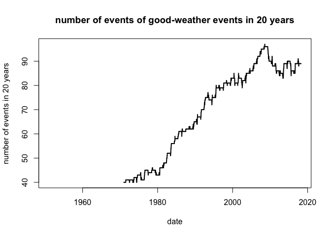
That is definitely a positive trend, probably due to the well-known positive trend of temperature over Europe and the Netherland. This is an example of how to use (free) observed data and some relatively simple code to try to understand the “weather” of a specific area. To this end, I would also suggest to keep an eye on the Copernicus Climate Change products, that are free for everyone and up-to-date.