From gridded data to time-series
Aggregating gridded data with Python and xarray
In the last years I needed many times to aggregate the data into a gridded dataset (for example ERA5 meteorological data) into a time-series, according to specific borders (for example administrative regions). In the past I was using a R package which I developed and that I used for example for the ERA-NUTS dataset. However, when recently I had to deal with a 5km resolution hydrological model (1M grid cells per day in Europe) I had to find a solution which allowed me to work out-of-memory. In this short post I will present a simple solution based on open-source Python modules:
- xarray: for manipulating & reading gridded data, and – very important – operate out-of-memory thanks to its dask capabilities
- regionmask: to mask a gridded file according to a shapefile
- numpy: for simple array manipulations
- geopandas: to open shapefiles
- matplotlib: for plotting
import xarray as xr
import numpy as np
import regionmask
import geopandas as gpd
import pandas as pd
import matplotlib.pyplot as plt
In this example we will use the NUTS classification developed by EUROSTAT. All the shapefiles are available on the EUROSTAT website. The files are available in different formats and in zipped archives containing multiple projections and spatialtypes: here I will use the file containing NUTS0 boundaries with EPSG:4326 projection and multipolygons as spatial type. The NUTS website provides all the needed information to choose the right files.
# Load the shapefile
PATH_TO_SHAPEFILE = 'shp/NUTS_RG_10M_2016_4326_LEVL_0.shp'
nuts = gpd.read_file(PATH_TO_SHAPEFILE)
nuts.head()
| LEVL_CODE | NUTS_ID | CNTR_CODE | NUTS_NAME | FID | geometry | |
|---|---|---|---|---|---|---|
| 0 | 0 | AL | AL | SHQIPËRIA | AL | POLYGON ((19.82698 42.4695, 19.83939 42.4695, ... |
| 1 | 0 | AT | AT | ÖSTERREICH | AT | POLYGON ((15.54245 48.9077, 15.75363 48.85218,... |
| 2 | 0 | BE | BE | BELGIQUE-BELGIË | BE | POLYGON ((5.10218 51.429, 5.0878 51.3823, 5.14... |
| 3 | 0 | NL | NL | NEDERLAND | NL | (POLYGON ((6.87491 53.40801, 6.91836 53.34529,... |
| 4 | 0 | PL | PL | POLSKA | PL | (POLYGON ((18.95003 54.35831, 19.35966 54.3723... |
nuts is a GeoDataFrame containing all polygons illustrating the national boundaries for the 37 countries in the NUTS classification.
Now we can load the gridded data. In a folder I hundreds of ERA5 reanalysis data downloaded from the CDS. Each of my files contains a single month of the global reanalysis, about 1.5 GB. The parameter chunks is very important, it defines how big are the “pieces” of data moved from the disk to the memory. With this value the entire computation on a workstation with 32 GB takes a couple of minutes.
I want to load all the temperature files for the year 2018. With the function assign_coords the longitude is converted from the 0-360 range to -180,180
# Read NetCDF
FOLDER_WITH_NETCDF = '/emhires-data/data-warehouse/gridded/ERA5/'
d = xr.open_mfdataset(FOLDER_WITH_NETCDF+'era5-hourly-2m_temperature-2018-*.nc', chunks = {'time': 10})
d = d.assign_coords(longitude=(((d.longitude + 180) % 360) - 180)).sortby('longitude')

d
<xarray.Dataset>
Dimensions:    (latitude: 721, longitude: 1440, time: 8760)
Coordinates:
  * longitude  (longitude) float32 -180.0 -179.75 -179.5 ... 179.25 179.5 179.75
  * latitude   (latitude) float32 90.0 89.75 89.5 89.25 ... -89.5 -89.75 -90.0
  * time       (time) datetime64[ns] 2018-01-01 ... 2018-12-31T23:00:00
Data variables:
    t2m        (time, latitude, longitude) float32 dask.array<shape=(8760, 721, 1440), chunksize=(10, 721, 1440)>
Attributes:
    Conventions:  CF-1.6
    history:      2019-04-27 23:33:00 GMT by grib_to_netcdf-2.10.0: /opt/ecmw...
As you can see this xarray Dataset contains a single variable (t2m) which is stored as a dask.array. This is the result of loading files with open_mfdataset. More information and examples of the interaction between dask and xarray can be found in their documentations(here and here)
Now we are ready for a bit of regionmask magic. The module can create a gridded mask with the function regions_cls documented here. With this function we have created an object able to mask gridded data.
# CALCULATE MASK
nuts_mask_poly = regionmask.Regions_cls(name = 'nuts_mask', numbers = list(range(0,37)), names = list(nuts.NUTS_ID), abbrevs = list(nuts.NUTS_ID), outlines = list(nuts.geometry.values[i] for i in range(0,37)))
print(nuts_mask_poly)
37 'nuts_mask' Regions ()
AL AT BE NL PL PT DK DE EL ES BG CH CY RO RS CZ EE HU HR SI SK SE IT TR FI NO IE IS LI LT LU LV ME MK UK MT FR
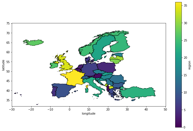
Now we are ready to apply the mask on the gridded dataset d. We select only the first timestep to speed up the process. For the same reason it is better to “zoom” only on the European continent. We specify the name of the coordinates (the defaults are lat and lon).
mask = nuts_mask_poly.mask(d.isel(time = 0).sel(latitude = slice(75, 32), longitude = slice(-30, 50)), lat_name='latitude', lon_name='longitude')
mask
<xarray.DataArray 'region' (latitude: 173, longitude: 321)>
array([[nan, nan, nan, ..., nan, nan, nan],
       [nan, nan, nan, ..., nan, nan, nan],
       [nan, nan, nan, ..., nan, nan, nan],
       ...,
       [nan, nan, nan, ..., nan, nan, nan],
       [nan, nan, nan, ..., nan, nan, nan],
       [nan, nan, nan, ..., nan, nan, nan]])
Coordinates:
  * latitude   (latitude) float32 75.0 74.75 74.5 74.25 ... 32.5 32.25 32.0
  * longitude  (longitude) float32 -30.0 -29.75 -29.5 -29.25 ... 49.5 49.75 50.0
The computation takes a couple of minutes but then the mask can be saved (for example as a NetCDF) for a later use.
plt.figure(figsize=(12,8))
ax = plt.axes()
mask.plot(ax = ax)
nuts.plot(ax = ax, alpha = 0.8, facecolor = 'none', lw = 1)
<matplotlib.axes._subplots.AxesSubplot at 0x7f362edea0b8>
Extract time-series
We can now for each country we would like to aggregate the grid cells in the national borders. The procedure is rather simple, I will focus on a single region and it is easy to extend it for multiple regions.
ID_REGION = 34
print(nuts.NUTS_ID[ID_REGION])
UK
As first step, I will save the latitude and longitude vectors because I will use it later. Then, I select the mask points where the value is equal to target value (the NUTS code). In the numpy array sel_mask all the values are nan except for the selected ones.
lat = mask.latitude.values
lon = mask.longitude.values


sel_mask = mask.where(mask == ID_REGION).values
sel_mask
array([[nan, nan, nan, ..., nan, nan, nan],
       [nan, nan, nan, ..., nan, nan, nan],
       [nan, nan, nan, ..., nan, nan, nan],
       ...,
       [nan, nan, nan, ..., nan, nan, nan],
       [nan, nan, nan, ..., nan, nan, nan],
       [nan, nan, nan, ..., nan, nan, nan]])
To speed-up the process I want to crop the xarray Dataset selecting the smallest box containing the entire mask. To do this I store in id_lon and id_lat the coordinate points where the mask has at least a non-nan value.
id_lon = lon[np.where(~np.all(np.isnan(sel_mask), axis=0))]
id_lat = lat[np.where(~np.all(np.isnan(sel_mask), axis=1))]
The d dataset is reduced selecting only the target year and the coordinates containing the target region. Then the dataset is load from the dask array using compute and then filtered using the mask. I came up with this procedure to speed up the computation and reduce the memory use for large dataset, apparently the where function is not really dask friendly.
out_sel = d.sel(latitude = slice(id_lat[0], id_lat[-1]), longitude = slice(id_lon[0], id_lon[-1])).compute().where(mask == ID_REGION)
out_sel
<xarray.Dataset>
Dimensions:    (latitude: 42, longitude: 39, time: 8760)
Coordinates:
  * latitude   (latitude) float64 60.5 60.25 60.0 59.75 ... 50.75 50.5 50.25
  * longitude  (longitude) float64 -8.0 -7.75 -7.5 -7.25 ... 0.75 1.0 1.25 1.5
  * time       (time) datetime64[ns] 2018-01-01 ... 2018-12-31T23:00:00
Data variables:
    t2m        (time, latitude, longitude) float32 nan nan nan ... nan nan nan
Attributes:
    Conventions:  CF-1.6
    history:      2019-04-27 23:33:00 GMT by grib_to_netcdf-2.10.0: /opt/ecmw...
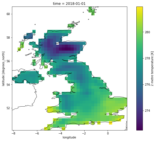
plt.figure(figsize=(12,8))
ax = plt.axes()
out_sel.t2m.isel(time = 0).plot(ax = ax)
nuts.plot(ax = ax, alpha = 0.8, facecolor = 'none')
<matplotlib.axes._subplots.AxesSubplot at 0x7f36285ff278>
Finally we can aggregate by the arithmetic mean using the groupby function to obtain a time-series of national average temperatures.
x = out_sel.groupby('time').mean()
x
<xarray.Dataset>
Dimensions:  (time: 8760)
Coordinates:
  * time     (time) datetime64[ns] 2018-01-01 ... 2018-12-31T23:00:00
Data variables:
    t2m      (time) float32 277.8664 277.64725 277.61978 ... 281.81863 281.60248
Then we plot the time-series…
x.t2m.plot()
[<matplotlib.lines.Line2D at 0x7f362e274518>]
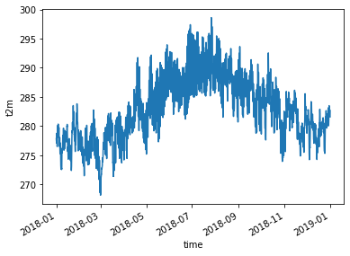
and we save it as a csv
x.t2m.to_pandas().to_csv('average-temperature.csv', header = ['t2m'])
The procedure is quite simple and can be definitely improved, for example adding a cosine weighting to a regular grid.